1.1. Modeling Events in UML and SysML

The UML standardization effort has been concerned with Object-Oriented (OO) modeling, but it has missed the modeling of events and the opportunity of modeling behavior/processes based on a general concept of events and their state changes. Instead, UML contributors have been obsessed with the computational concept of state machines requiring to name all relevant states of an object, which is an approach that does not scale.

It is rather strange that even in OMG’s new Kernel Modeling Language, the behavior/process modeling concepts of Behaviors and Interactions are defined without even mentioning the term “event”.

Olivé and Raventós (2006) presume that in UML, events have not been considered as first-class citizens (as instances of event classes), but rather in the limited form of operation invocations, due to the desire to separate “structural modeling” from “behavioral modeling”.

The UML-based System Modeling Language (SysML) allows modeling “blocks” (representing system components), which can be connected via “ports” for allowing data flows and signal flows between “blocks”.

UML/SysML limit the concept of events to specific uses in State Machine Diagrams and Activity Diagrams (“Call Event”,”Change Event”,”Signal Event”,”Time Event”). Unlike OEM, UML/SysML do not support a general concept of events, which would include UI events and business events.

1.2. Related Work

Unlike in the field of DES, in the field of IS engineering the idea of modeling events as entities in information models and combining this with modeling objects is not new. Already Peter Chen (1976), in his seminal paper proposing Entity-Relationship (E-R) modeling, suggested that both objects and events should be modelled as entities: “A specific person, company, or event is an example of an entity”. Motivated by the importance of events such as sales, purchases, or cash receipts, in accounting, McCarthy (1979) has proposed to model these events, along with objects, as entities in E-R models  However, neither Chen nor McCarthy considered the fundamental semantic differences between these two kinds of entities and treated them in the same way.

Independently of each other, Allen and March (2003) as well as Olivé and Raventós (2006) have proposed modeling events as entities in information models taking into consideration how they affect the state of objects.

Allen and March (2003) propose to include the events responsible for object state changes as entities in an E-R model arguing that this approach is preferable to temporal database approaches whenever temporality is needed. March and Allen (2009), by stating that “an information system must be conceptualized as an event-processing mechanism and an event as the cause of the transition from an initial state to a subsequent state via the application of its rules”, already have been aware of the concept of event rules as transition functions, which is the basis of the semantics of DPMN process models (Wagner 2017).

Olivé and Raventós (2006) propose modelling events as entities and event types as classes with a special effect() operation in UML class models. Their effect() operation essentially corresponds to the OEM concept of event rules, or the event handlers onEvent() and onActivityEnd() in OEMjs. Olivé and Raventós integrate information and behavior/process modeling in their extended form of UML class diagrams. However, it seems preferable to separate behavior/process modeling from information modeling. While the latter is in charge of defining the types of objects, events and activities (including their attributes, associations, operations and constraints), the former is in charge of defining event rules, which define the effects of events and the admissible sequences of events.

Neither Allen and March nor Olivé and Raventós have made a distinction between instantaneous events and activities.

2.1. Making Conceptual Information Models

A conceptual information model describes the subject matter vocabulary used, e.g., in the system narrative, in a semi-formal way. Such a vocabulary essentially consists of names for

• types, corresponding to classes in OO modeling, or unary predicates in formal logic,
• properties, corresponding to binary predicates in formal logic,
• associations, corresponding to n-ary predicates (with n > 1) in formal logic.

The main categories of types are object types and event types. A simple form of conceptual information model is obtained by providing a list of each of them, while a more elaborated model, e.g., in the form of a UML class diagram, also defines properties and associations, including those that describe the participation of objects (of certain types) in events (of certain types).

2.1.1. Modeling Object Types

Object types are modeled in OE class diagrams in the form of class rectangles categorized with the ("stereotype") keyword «object type».

As an illustrating example, consider a public library, which lends book copies to its users. For this organization, the most important object types are Book, BookCopy, Person, and LibraryUser, as described by the following class diagram:

This model includes two associations and one generalization:

1. The many-to-one association between book copy and book associating exactly one book with any book copy (and, inversely, zero to many book copies with any book).
2. The many-to-many association between book and person associating zero to many people as authors with a book (and, inversely, zero to many books with any person as one of their authors).
3. The generalization from library user to person stating that any library user is also a person and, hence, has the attributes id, name, birth date and biography.

2.1.2. Modeling Event Types

For simplicity, we often say "event" instead of "instantaneous event". We trust the reader's ability to disambiguate the intended meaning of "event": either denoting the general category of events or the specific category of instantaneous events.

All event types have the implicit attributes startTime, occurrenceTime, and duration, where duration = occurrenceTime − startTime. For instantaneous events, such as user arrivals and departures, only their occurrence time is meaningful, they don't have a start time and a duration.

It is important to understand that objects participate in events – this is a principle of foundational ontologies such as UFO. This implies that there are corresponding participation associations between an event type and its participating object types.

Event types are modeled in Object Event (OE) class diagrams in the form of class rectangles categorized with the ("stereotype") keyword «event type», as shown in the following example model:

This model includes the four event types arrival, departure, book borrowing and book return. While arrival and departure events have a library user as their only participating object, book borrowing and book return events have both a library user and one or more book copies as participants.

Notice that book borrowing and book return events represent corresponding activity end events since borrowing and returning books are, in fact, activities that take some time and, therefore, consist of an activity start event followed by an activity end event. Whenever we are not interested in considering their start event and their duration, we can reduce activities to their (instantaneous) end events, as in the model above.

Due to the temporal snapshot semantics of UML class models, according to the multiplicity 0..1 at the Arrival association end, a library user participates in at most one current Arrival event, although there may be many past/historic Arrival events, in which that user has participated and we assume that an IS stores these historic event records in its database.

For supporting a distinction between snapshot and history cardinality constraints, Tauzovich (1991) has proposed to add a “lifetime cardinality” as a supplement to the snapshot cardinality to association ends in his Temporal Entity-Relationship modeling approach. We adopt this distinction for OE class models, where we allow for a history multiplicity expression in the form of “H:m“, where m is a normal multiplicity expression (such as * or 0..1), in addition to the standard snapshot multiplicity expression at the event/activity class side (or association end) of a participation association. For avoiding the cluttering of OE class diagrams, we assume that, by default, at the event/activity class side of a participation association, the snapshot multiplicity is 0..1 and the history multiplicity is *, so explicit expressions for these two multiplicities only have to be displayed if they differ from these defaults.

2.1.3. Modeling Activity Types

Activity types have the implicit attributes startTime, occurrenceTime, and duration, where duration = occurrenceTime − startTime. Activities occur when they end/complete.

Activity types are modeled in OE class diagrams in the form of class rectangles categorized with the ("stereotype") keyword «activity type», as shown in the following example model:

This model includes the two activity types BookLending and BookTakeBack, both of which have a library user and one or more book copies as their participating objects.

2.2. Making Conceptual Process Models

A conceptual process model should describe a causal regularity in the form of an event rule, for each type of events identified in the conceptual information model. This includes describing in which temporal sequences events may occur, based on conditional and parallel branching. A conceptual event rule for an event type describes the state changes and follow-up events caused by events of that type.

A conceptual process model can be expressed textually in the form of a list or a table of event rule statements or visually in the form of an Object Event Graph or a DPMN Process Diagram.

2.2.2. Conceptual Modeling of Causal Regularities with Object Event Graphs

Object Event Graphs (OEGs) extend the Event Graph diagram language by adding object rectangles containing declarations of typed object variables and state change statements, as well as gateway diamonds for expressing conditional and parallel branching.

The following OEG is based on the object and event type definitions of the OE class diagram shown in .

2.2.3. Conceptual Modeling of Causal Regularities with Activity Networks

Object Event Graphs (OEGs) extend the Event Graph diagram language by adding object rectangles containing declarations of typed object variables and state change statements, as well as gateway diamonds for expressing conditional and parallel branching.

The following OEG is based on the object, event and activity type definitions of the OE class diagram shown in .

This model includes the two activity types BookLending and BookTakeBack, both of which have a library user and one or more book copies as their participating objects.

3.1. Designing Information Systems

For designing an information system (IS), it is essential to identify the types of business objects, business events and business activities that have to be represented and supported by the IS. This choice can be made on the basis of the conceptual domain model and the IS requirements provided by the project clients. In the case of our example problem, the public library, these types are:

1. the business object types Book, BookCopy, LibraryUser and Person;
2. the business event types Arrival and Departure;
3. business activity types BookLending and BookTakeBack.

Notice that in the design model, as is common in OO modeling, we use camel case notation for all type names.

3.1.1. Making Information Design Models for IS Engineering

An information design model is derived from a conceptual information model by choosing the design-relevant types of objects and events and enrich them with design details, while dropping other object types and event types not deemed relevant for the simulation design. Adding design details includes specifying property ranges as well as adding multiplicity and other types of constraints.

As opposed to the underlying conceptual information model shown in Section 2.1.3, the following information design model provides attribute ranges, standard identifier, mandatory value and key constraint declarations (by default, in UML, attributes are mandatory and single-valued).

Notice also the notation "/date" in the attribute compartments of the activity classes BookLending and BookTakeBack, where the slash prefix indicates that the attribute date is a derived attribute (its value can be automatically computed from the implicit occurrenceTime attribute).

3.1.2. Making Process Design Models for IS Engineering

In a process design model for a process-supportive IS, we refine a conceptual process model by adding all details needed for obtaining a computationally complete definition of the business processes to be supported. An important question is whether these processes consist of activities that have to be performed in a certain order, like workflow processes, or that may be performed in any order, like flexible business processes. In the former case, the workflow sequencing of activities has to be defined in a suitable process model, while in the latter case, workflow sequencing is not needed and it is sufficient to define the state changes that come with the performance of activities.

In our example of a public library process shown in the following conceptual process model diagram, there are only two types of activities, book lending and book take back, which may be performed in any order.

Notice that the sequencing from arrival events to book lending and book take back activities in this conceptual process model does not mean that there is a corresponding workflow sequencing such that on arrival, a book lending or book take back activity can be scheduled in the task list of the library clerk in charge. Rather, since the start times of any book lending and book take back activities are controlled by the library user going to the service desk, and not by the library clerk, there is no workflow sequencing and, consequently, we have to drop the work sequence flow arrows in the process design model, as shown in the following diagram:

This process design model, using the names (of types, attributes and operations) defined in the information design model shown in Section 3.1.1, defines in the attached object rectangles for all event circles and activity rectangles:

1. variable names and bindings of these variables to parameter values (e.g., by the equality u = a.user assigning the user object reference of the expression a.user to the variable u),
2. state change statements that will be executed when a corresponding event occurs or when a corresponding activity completes.

Since these variable definitions and state change statements can also be expressed in onEvent and onActivityEnd operations in corresponding event and activity classes, they can be added to the OE class model from Section 3.2.1 by adding these operations resulting in the following model:

3.2. Designing Discrete Event Simulations

A simulation design model defines a computational design for a simulation based on a conceptual model. Unlike the conceptual model, the design is tailored towards the purpose of the simulation project (e.g., for answering certain research questions in a social system analysis project or in a technical system engineering project, or for teaching certain facts about a system in an educational simulation project). Although the design model is independent of a specific technology platform, it is typically based on OO modeling (e.g., with UML diagrams). It can be implemented in different ways with any specific technology choice, typically using an OO programming approach.

3.2.1. Making Information Design Models for DES Engineering

In addition to the general information modeling issues, there are also a few issues, which are specific for simulation modeling:

1. The information design model must designate attributes representing state variables that are subject to random variation, so they can be considered as random variables with an underlying probability distribution that is sampled by a corresponding method stereotyped «rv» for categorizing it as a random variate sampling method. The underlying probability distribution can be indicated in the model diagram by appending a symbolic expression, denoting a distribution (with parameter values), to the method definition clause. For instance, U(1,6) may denote the uniform distribution with lower bound 1 and upper bound 6, while Exp(1.5) may denote the exponential distribution with event rate 1.5.
2. The information design model must distinguish between exogenous and caused (or endogenous) event types. For any exogenous event type, the recurrence of events of that type must be specified, typically in the form of a random variable, but in some cases it may be a constant (like 'on each Monday'). The recurrence defines the elapsed time between two consecutive events of the given type (their inter-occurrence time). It can be specified within the event class concerned in the form of a special operation with the predefined name 'recurrence' and normally annotated with a probability distribution expression.
3. The information design model must add a duration() function to all activity classes. This function is invoked when a new activity is created for computing the value of its duration attribute. Normally, the duration() function represents a random variable, to be indicated by appending a probability distribution annotation such as Exp(1.5).
4. If the simulation is to deal with objects in space, the design model must be based on a choice of space model: one-dimensional (1D) discrete space, two-dimensional (2D) discrete space (also called grid space), three-dimensional (3D) discrete space, and 1D/2D/3D continuous space. The chosen space model implies a corresponding form of spatial positions (or locations): a 1-, 2- or 3-tuple of integers or decimal numbers.

Following these rules, by extending the IS information design model (from Section 3.1.1) we obtain the following model:

3.2.2. Making Process Design Models for DES Engineering

In a process simulation design model, we refine a conceptual process model by adding all details needed for obtaining a computationally complete process simulation model that can be directly transformed into simulation code.

4.1. The ES Formalism

We illustrate the formal semantics of ES with the help of an example. We model a system of one or more service desks, each of them having its own queue, as a discrete event system characterized by the following narrative:

1. Customers arrive at a service desk at random times.
2. If there is no other customer in front of them, and the service desk is available, they are served immediately, otherwise they have to queue up in a waiting line.
3. The duration of services varies, depending on the individual case.
4. When a service is completed, the customer departs and the next customer is served, if there is still any customer in the queue.

The base concepts of ES are:

1. state variables for describing the state of a system,
2. event types,
3. event expressions,
4. event routines,
5. future events lists (FEL).

A state variable is declared with a name and a range, which is a datatype defining its possible values.

An event type is defined in the form of a class: with a name, a set of property declarations and a set of method definitions, which together define the signature of the event type.

An event expression is a term E(x)@t where

1. E is an event type,
2. t is a parameter for the occurrence time of events,
3. x is a (possibly empty) list of event parameters x₁, x₂, …, x_n according to the signature of the event type E.

For instance, Arrival@t is an event expression for describing Arrival events where the signature of the event type Arrival is empty, so there are no event parameters, and the parameter t denotes the arrival time (more precisely, the occurrence time of the Arrival event). An individual event of type E is a ground event expression, e = E(v)@i, where the event parameter list x and the occurrence time parameter t have been instantiated with a corresponding value list v and a specific time instant i. For instance, Arrival@1 is a ground event expression representing an individual Arrival event.

An event rule associates an event expression with an event routine F:

ON E(x)@t DO F( t, x),

where the event expression E(x)@t specifies the type E of events that trigger the rule, and F( t, x) is a function call expression for computing a set of state changes and a set of follow-up events, based on the event parameter values x, the event's occurrence time t and the current system state, which is accessed in the event routine F for testing conditions expressed in terms of state variables.

A Future Events List (FEL) is a set of ground event expressions partially ordered by their occurrence times, which represent future time instants either from a discrete or a continuous model of time. The partial order implies the possibility of simultaneous events, as in the example { Departure@4, Arrival@4 }.

4.2. Event Graphs

Event Graphs (EGs) have been proposed as a diagram language for making ES models by Schruben (1983). A node in an EG is visually rendered as a circle and represents a typed event variable (such that the node's name is the name of the associated event type). An event circle may be annotated with state change statements in the form of state variable assignments. An arrow (or directed edge) between two event circles (nodes) represents (a) the causation of a follow-up event in the case of a conceptual process model, or (b) the scheduling of a follow-up event according to the event scheduling paradigm in the case of a process simulation design model.

An Event Graph defining an ES model for a service desk system with one state variable (Q for queue length) and two event types (Arrival and Departure) is shown in the following diagram:

This model specifies three event rules, one for each event circle:

1. On each initial event (the leftmost unnamed circle), the variable Q is initialized by setting it to 0, and then an Arrival event is scheduled to occur immediately.
2. When an Arrival event occurs, the variable Q is incremented by 1 and, if Q is equal to 1, a Departure event is scheduled with a delay provided by invoking the function serviceTime (representing a random variable); in addition (since Arrival events are exogenous), a new Arrival event is scheduled with a delay provided by invoking the function recurrence (also representing a random variable).
3. When a Departure event occurs, the variable Q is decremented by 1 and, if Q is greater than 0 (that is, if the queue is non-empty), another Departure event is scheduled with a delay provided by invoking the function serviceTime.

In Schruben's original notation for EGs used above:

1. There is an initial event (the left-most unnamed circle in the example EG above) creating the initial state with the help of one or more initial state variable assignments (here Q := 0) and triggering the real start event (here: Arrival). In our improved notation for EGs, we will drop this element in favor of getting simpler diagrams and assume that the initial state definition is taken care of separately and is not part of a process model diagram.

2. The recurrence of a start event (here: Arrival) is explicitly modeled with the help of a recursive arrow (going from the Arrival event circle to the Arrival event circle). In our improved notation for EGs, this recursive arrow is dropped assuming that the type definition of exogenous start events includes a recurrence function that is invoked by a simulator for automatically scheduling recurrent exogenous events (like Arrival).

3. Conditional event scheduling arrows are indicated by annotating the arrows with a condition in parenthesis, as shown above for the arrow between Arrival and Departure and the (reverse) arrow between Departure and Arrival. In our improved notation for EGs, we replace the parenthesis with brackets and use BPMN's notation for conditional "sequence flow" arrows with a mini-diamond at the arrow's start as shown below.

The same service desk model is shown in the following diagram using the improved notation resulting from these three simplifications/modifications:

Notice that in our improved notation for EGs, we use a prefix "+" for delay expressions, e.g., writing "+serviceTime()" instead of "serviceTime()" as an annotation of the event scheduling arrow between Arrival and Departure, for better indicating that the expression represents a scheduling delay. Notice also that, to a great extent, we use the visual notation of BPMN, but not its semantics (e.g., we do not use BPMN's visual distinction between "Start" and "Intermediate" events).

EGs provide a visual modeling language with a precise semantics that captures the fundamental event scheduling paradigm. However, EGs are a rather low-level DES modeling language: they lack a visual notation for (conditional and parallel) branching, do not support object-oriented state structure modeling (with attributes of objects taking the role of state variables) and do not support the concept of activities.

Formally, an EG is defined on the basis of a set of event types ET and a set of state variables V as a directed graph ⟨ N, D ⟩ with nodes N and directed edges D ⊆ N ⨉ N , such that

1. each node n ∈ N is associated with

   1. an event type E ∈ ET,
   2. an event variable e representing an event of type E,
   3. a (possibly empty) set of variable value assignments of the form v := expr with v ∈ V and an expression expr formed with the help of the event variable e and variables from V, defining an on-event state transition function;
2. each directed edge ⟨ n₁, n₂ ⟩ ∈ D may be associated with
   1. a numeric delay expression δ possibly expressed with the help of the event variable e and variables from V,
   2. a condition (or Boolean expression) C expressed with the help of the event variable e and variables from V.

5.1. The OES Formalism

The OEM&S paradigm is based on the OES formalism presented in (Wagner 2017), which is summarized below.

A set of object types OT defines a predicate-logical signature as the basis of a logical expression language L_OT: each object type defines a unary predicate, and its properties define binary predicates. A state change language C_OT based on OT defines state change statements expressed with the help of the object type names and property names defined by OT. In the simplest case, state change statements are property value assignments like o.p₁ := 4 or o.p₁ := o.p₂ where o is an object variable and p₁, p₂ are property names.

A set of objects O = {o₁, o₂, ...o_n} where each of them has a state in the form of a set of slots (property-value pairs) represents a system state, that is a state of the real-world system being modeled and simulated. A system state O can be updated by a set of state changes (or, more precisely, state change statements) Δ ⊆ C_OT with the help of an update operation Upd. For instance, for a system state O₁ = {o₁} with o₁ = { p₁: 2, p₂: 5} and a set of state changes Δ₁ = { o₁.p₁ := o₁.p₂ } we obtain

An event expression is a term E(x)@t where

1. E is an event type,
2. x is a (possibly empty) list of event parameters x₁, x₂, …, x_n according to the signature of the event type E,
3. t is a parameter for the occurrence time of events.

For instance, PartArrival(ws)@t is an event expression for describing part arrival events where the event parameter ws is of type WorkStation, and t denotes the arrival time. An individual event of type E is a ground event expression, e = E(v)@i, where the event parameter list x and the occurrence time parameter t have been instantiated with a corresponding value list v and a specific time instant i. For instance, PartArrival(ws1)@1 is a ground event expression representing an individual PartArrival event occurring at workstation ws1 at time 1.

An event routine is a procedure that essentially computes state changes and follow-up events, possibly based on conditions on the current state. In practice, state changes are often directly performed by immediately updating the objects concerned, and follow-up events are immediately scheduled by adding them to the FEL. For the OES formalism, we assume that an event routine is a pure function that computes state changes and follow-up events, but does not apply them, as illustrated by the examples in the following table.

An event rule associates an event expression with an event routine F:

where the event expression E(x)@t specifies the type E of events that trigger the rule, and F( t, x) is a function call expression for computing a set of state changes and a set of follow-up events, based on the event parameter values x, the event's occurrence time t and the current system state, which is accessed in the event routine F for testing conditions expressed in terms of state variables.

An OE model based on a state change language C_OT and a corresponding update operation Upd is a triple ⟨OT, ET, R⟩, consisting of a set of object types OT, event types ET and event rules R.

An event rule r = ON E(x)@t DO F( t, x) can be considered as a 2-step function that, in the first step, maps an event e = E(v)@i to a parameter-free state change function r_e = F( i, v), which maps a system state O to a pair ⟨ Δ, FE ⟩ of system state changes Δ ⊆ C_OT and follow-up events FE. When the parameters t and x of F( t, x) are replaced by the values i and v provided by a ground event expression E(v)@i, we also simply write F_i,v instead of F( i, v) for the resulting parameter-free state change function.

We say that an event rule r is triggered by an event e when the event's type is the same as the rule's event type. When r is triggered by e, we can form the state change function r_e = F_i,v and apply it to a system state O by mapping it to a set of state changes and a set of follow-up events:

We can illustrate this with the help of our workstation example. Consider the rule r_PA defined in the table above triggered by the event PartArrival(ws1)@1 in state O₀ = {ws1.status: AVAILABLE, ws1.waitingParts: []}. We obtain

with Δ₁ = { ws1.waitingParts.push( a.part)} and FE₁ = {ProcessingStart@2}.

An OE model defines a state transition system where

1. A state is a simulation state S = ⟨t, O, E⟩.

2. A transition of a simulation state S consists of

   1. advancing t to the occurrence time t' of the next events NE ⊆ E, which is the set of all imminent events with minimal occurrence time;

   2. processing all next events e ∈ NE by applying the event rules r ∈ R triggered by them to the current system state O according to

      r_e( O ) = ⟨ Δ_e , FE_e ⟩

      resulting in a set of state changes Δ = ∪ {Δ_e | e ∈ NE } and a set of follow-up events FE = ∪ {FE_e | e ∈ NE }.

   such that the resulting successor simulation state is S' = ⟨ t', O', E' ⟩ with O' = Upd( O, Δ) and E' = E − NE ∪ FE.

Notice that the OES formalism first collects all state changes brought about by all the simultaneous next events (from the set NE) of a simulation step before applying them. This prevents the state changes brought about by one event from NE to affect the application of event rules for other events from NE, thus avoiding the problem of non-determinism through the potential non-confluence (or non-serializability) of parallel events.

OE simulators are computer programs that implement the OES formalism. Typically, for performance reasons, discrete event simulators do not first collect all state changes brought about by all the simultaneous next events (the set NE) of a simulation step before applying them, but rather apply them immediately in each triggered event routine. However, this approach takes the risk of an unreliable semantics of certain simulation models in favor of performance.

5.2. Object Event Graphs

The following basic DPMN diagram shows an OEG defining a process pattern that is instantiated by the above discrete event process example.

This process model is based on the following Object Event (OE) class model:

Notice that the multiplicity 1 (standing for "exactly one") at the association end touching the object class WorkStation expresses the constraint that exactly one workstation must participate in any event of one of the associated types (PartArrival, ProcessingStart, or ProcessingEnd), while the multiplicity 0..1 (standing for "at most one") at the other association ends (touching one of the three event classes) expresses the constraint that, at any moment, a workstation participates in at most one PartArrival event, in at most one ProcessingStart event, and in at most one ProcessingEnd event. Notice that a further constraint should be added: at any moment, a workstation must not participate in both a ProcessingStart and a ProcessingEnd event.

An OEG specifies a set of chained event rules, one rule for each event circle of the model. The above OEG specifies the following three event rules:

1. On each PartArrival event, the inputBufferLength attribute of the associated WorkStation object is incremented and if the workstation's status attribute has the value AVAILABLE, then a new ProcessingStart event is scheduled to occur immediately.
2. When a ProcessingStart event occurs, the associated WorkStation object's status attribute is changed to BUSY and a ProcessingEnd event is scheduled with a delay provided by invoking the processingTime function defined in the ProcessingStart event class.
3. When a ProcessingEnd event occurs, the inputBufferLength attribute of the associated WorkStation object is decremented and if the inputBufferLength attribute has the value 0, the associated WorkStation object's status attribute is changed to AVAILABLE. If the inputBufferLength attribute has a value greater than 0, a new ProcessingStart event is scheduled to occur immediately.

The formal (transition system) semantics of OEGs, based on the semantics of event rules as transition functions, has been presented in (Wagner 2017). It can be shown that the OEG diagram language is a conservative extension of the Event Graph diagram language by means of a homomorphic embedding of Event Graphs in OEGs.

Formally, an OEG is defined on the basis of a set of object types OT and a set of event types ET as a directed graph ⟨ N, D ⟩ with nodes N and directed edges D ⊆ N ⨉ N , such that

1. each node n ∈ N is associated with

   1. an event type E ∈ ET with event participation roles P_E,
   2. an event variable e representing an event of type E,
   3. a (possibly empty) set of auxiliary (shortcut) object variables o defined with the help of event participation roles p ∈ P_E by setting o := e.p,
   4. a (possibly empty) set of definitions of on-event object state transition functions { f_p | p ∈ P_E };
2. each directed edge ⟨ n₁, n₂ ⟩ ∈ D may be associated with
   1. a numeric delay expression δ possibly expressed with the help of the variables associated with n₁,
   2. a condition (or Boolean expression) C expressed with the help of the variables associated with n₁.

6.1. Conceptual Modeling of Simple Activities

Conceptually, an activity is a composite event that is composed of, and temporally framed by, a pair of start and end events. Consequently, whenever a model contains a pair of related start and end event types, like processing start and processing end in the model of a manufacturing workstation shown on the left-hand side of Figure 6-1 and Figure 6-2, they can be replaced with a corresponding activity type, like processing, as shown on the right-hand side.

It is obvious that applying this replacement pattern leads to a conceptual and visual simplification of the models concerned.

6.2. Design Modeling of Simple Activities

Like in a conceptual model, also in a design model, a pair of corresponding activity start event and end event circles, like ProcessingStart and ProcessingEnd in the source models shown in Figure 6-3 and Figure 6-4, can be replaced with a corresponding activity rectangle, like Processing, as in the target models shown in these figures.

Extending basic OE class design models by adding activity types

In the case of an OE class design model, this replacement pattern implies allocating all features (attributes, associations and operations) of the classes defining the start and the end event type in the class defining the corresponding activity type, possibly with renaming some of them. In the example of Figure 6-3, there is only one such feature: the class-level operation ProcessingStart::processingTime, which is allocated to Processing and renamed to time.

Extending Object Event Graphs by adding Activity rectangles

In the case of a process design model, the rewrite pattern implies that an Event circle pair consisting of an Event circle intended to represent activity start events and an Event circle intended to represent related activity end events, with an event scheduling arrow from the start to the end Event circle annotated by a delay expression, is replaced by an Activity rectangle such that:

1. All Data Objects attached to the end Event circle get attached to the Activity rectangle (since an activity occurs when it it is completed).
2. All event scheduling arrows going out from the end Event circle are turned into event scheduling arrows going out from the Activity rectangle.
3. All start event scheduling arrows are replaced with corresponding activity scheduling arrows having an additional creation parameter assignment for the duration of a scheduled activity, which is set to the delay expression defined for the end event scheduling arrow. In the example above, the duration parameter in the annotation of the two activity scheduling arrows is set to Processing::time() in the target diagram, which is the same as the delay ProcessingStart::processingTime in the source diagram.
4. When the start Event circle has one or more attached Data Objects or any outgoing event scheduling arrow that does not go to the end Event circle, then a start Event circle has to be included in the Activity rectangle for attaching the Data Object(s) and as the source of the outgoing event scheduling arrow(s).

This Activity-Start-End Rewrite Pattern, which can also be applied in the inverse direction, replacing an Activity rectangle with an Event circle pair, defines the meaning of an Activity rectangle in a DPMN diagram. It allows reducing a DPMN-A diagram with Activity rectangles to an Object Event Graph (a basic DPMN diagram without Activity rectangles).

Notice that, like the source model, also the target model of Figure 6-4 specifies three event rules:

1. On each PartArrival event, the arrived part is added to the workstation's input buffer and if the workstation's status is AVAILABLE, then a new Processing activity is scheduled to start immediately with a duration provided by invoking the time function defined in the Processing activity class.
2. When a Processing activity starts, the workstation's status is changed to BUSY.
3. When a Processing activity ends, the processed part is removed from the input buffer and, if the input buffer is not empty, a new Processing activity is scheduled to start immediately, otherwise (if the input buffer is empty) the workstation's status is changed to AVAILABLE.

An alternative process design model of the single workstation system

Based on the same information design model, shown in the target model of Figure 6-3, we can make another process design model of the single workstation system as an alternative to the target model of Figure 6-4. This alternative model makes it more clear that a workstation is, in fact, an exclusive resource of its processing activity. The concepts of resources and resource-constrained activities are discussed in the following sections, and in Section 7.2, it is shown how to simplify the basic DPMN model of Figure 6-5 by using the higher-level modeling elements introduced in DPMN-A.

7.1. Conceptual Modeling of Resource-Constrained Activities

In the DES paradigm of Processing Networks, Gordon (1961) has introduced the resource management operations Seize and Release in the simulation language GPSS for allocating and de-allocating (releasing) resources. Thus, GPSS has established a standard modeling pattern for resource-constrained activities, which has become popular under the name of Seize-Delay-Release indicating that for simulating a resource-constrained activity, its resources are first allocated ("seized"), and then, after some delay representing the duration of the simulated activity, they are de-allocated ("released").

Resource roles, process owners and resource pools

As an illustrative example, we consider a hospital consisting of medical departments where patients arrive for getting a medical examination performed by a doctor. A medical examination, as an activity, has three participants: a patient, a medical department, and a doctor, but only one of them plays a resource role: doctors. This can be indicated in an OE Class Diagram by using the stereotype «resource role» for categorizing the association ends that represent resource roles, as shown in Figure 7-3.

Notice that both the event type patient arrivals and the activity type examinations have a (mandatory functional) reference property process owner. This implies that both patient arrival events and examination activities happen at a specific medical department, which is their process owner in the sense that it owns the process types composed of them. A process owner is called "Participant" in BPMN (in the sense of a collaboration participant) and visually rendered in the form of a container rectangle called "Pool".

In Figure 7-3, the resource role of doctors corresponds to the performer role. In BPMN, Performer is considered to be a special type of resource role. According to (BPMN 2011), a performer can be "a specific individual, a group, an organization role or position, or an organization".[1]In BPMN, Performer is specialized into the HumanPerformer of an activity, which is, in turn, specialized into PotentialOwner denoting the "persons who can claim and work" on an activity of a given type. "A potential owner becomes the actual owner [...] by explicitly claiming" an activity. Allocating a human resource to an activity by leaving the choice to those humans that play a suitable resource role is characteristic for workflow management systems, while in traditional DES approaches to resource handling, as in Arena, Simio and AnyLogic, (human) resources are assigned to a task (as its performer) based on certain policies.

Thus, the term "performer" subsumes several types of performers. We will, by default, use it in the sense of a human performer.

One of the main reasons for considering certain objects as resources is the need to collect utilization statistics (either in an operational information system, like a workflow management system, or in a simulation model) by recording the use of resources over time (their utilization) per activity type. By designating resource roles in information models, these models provide the information needed in simulations and information systems for automatically collecting utilization statistics.

In the hospital example, a medical department, as the process owner, is the organizational unit that is responsible for reacting to certain events (here: patient arrivals) and managing the performance of certain processes and activities (here: medical examinations), including the allocation of resources to these processes and activities. For being able to allocate resources to activities, a process owner needs to manage resource pools, normally one for each resource role of each type of activity (if pools are not shared among resource roles). A resource pool is a collection of resource objects of a certain type. For instance, the three X-ray rooms of a diagnostic imaging department form a resource pool of that department.

Resource pools can be modeled in an OE Class Diagram by means of special associations between object classes representing process owners (like medical departments) and resource classes (like doctors), where the association ends, corresponding to collection-valued properties representing resource pools, are stereotyped with «resource pool», as shown in Figure 7-3. At any point in time, the resource objects of a resource pool may be out of order (like a defective machine or a doctor who is not on schedule), busy or available.

A process owner has special procedures for allocating available resources from resource pools to activities. For instance, in the model of Figure 7-3, a medical department has the procedure "allocate a doctor" for allocating a doctor to a medical examination. These resource allocation procedures may use various policies, especially for allocating human resources, such as first determining the suitability of potential resources (e.g., based on expertise, experience and previous performance), then ranking them and finally selecting from the most suitable ones (at random or based on their turn). See also (Arias et al 2018).

The conceptual process model shown in Figure 7-4 is based on the information model above. It refers to a medical department as the process owner, visualized in the form of a Pool container rectangle, and to doctor objects, as well as to the event type patient arrivals and to the activity type examinations.

This process model describes two causal regularities in the form of the following two event rules, each stated with two bullet points: one for describing all the state changes and one for describing all the follow-up events brought about by applying the rule.

1. When a new patient arrives:

   • if a doctor is available, then she is allocated to the examination of that patient; otherwise, a new planned examination is queued up;
   • if a doctor has been allocated, then start an examination of the patient.

2. When an examination is completed by a doctor:

   • if the queue of planned examinations is empty, then the doctor is released;
   • otherwise, the next planned examination by that doctor is scheduled to start immediately.

These conceptual event rules describe the real-world dynamics of a medical department according to business process management decisions. Changes of the waiting line and (de-)allocations of doctors are considered to be state changes (in the, not necessarily computerized, information system) of the department, as they are expressed in Data Object rectangles, which represent state changes of affected objects caused by an event in DPMN.

Notice that the model of Figure 7-4 abstracts away from the fact that after allocating a doctor, patients first need to walk to the room before their examination can start. Such a simplification may be justified if the walking time can be neglected or if there is no need to maximize the productive utilization of doctors who, according to this process model, have to wait until the patient arrives at the room. Below, this model is extended for allowing to allocate rooms and doctors such that patients have to wait for doctors, and not the other way around.

Switching roles: doctors as patients

The same person who is a doctor at a diagnostic imaging department may be treated as a patient of that department. It's a well-known fact that in the real world people may switch roles and may play several roles at the same time, but many modeling approaches/platforms fail to admit this. For instance, the simulation language (SIMAN) of the well-known DES modeling tool Arena does not treat resources and processing objects ("entities") as roles, but as strictly separate categories. This language design decision was a meta-modeling mistake, as admitted by Denis Pegden, the main creator of SIMAN/Arena, in (Drogoul et al 2018) where he says "it was a conceptualization mistake to view Entities and Resources as different constructs".

In Figure 7-5, the above model is extended by categorizing the classes doctors and patients as «role type» classes and adding the «kind» class people as a supertype of doctors and patients, we create the possibility that a person may play both roles: the role of a doctor and the role of a patient, albeit not at the same time. The object type categories «kind» and «role type» have been introduced to conceptual modeling by Guizzardi (2005).

Decoupling the allocation of multiple resources

For being more realistic, we consider the fact that patients first need to be walked by nurses to the room allocated to their examination before the examination can start. Thus, in the model of Figure 7-6, we add a second activity type, walks to room, involving people (typically, nurses and patients) walking to an examination room.

This process model describes three causal regularities in the form of the following three event rules:

1. When a new patient arrives:

   • if a room and a nurse are available, they are allocated to the walk of that patient to that room, otherwise a new planned walk is placed in the corresponding queue;
   • if a room has been allocated, then the nurse starts walking the patient to the room.

2. When a walk of a patient and nurse to a room is completed:

   • if there is still a planned walk in the queue and a room is available, then the room is allocated and the nurse is re-allocated to the walk of the next patient to that room.
     if a doctor is available, she is allocated to the examination of that patient, else a new planned examination of that patient is queued up;
   • if a doctor has been allocated, then the examination of that patient starts
     if the nurse has been re-allocated, she starts walking the next patient to the allocated room.

3. When an examination of a patient is completed by a doctor in a particular room:

   • if there is still a planned examination (of another patient in another room), then re-allocate the doctor to that planned examination, else release the doctor;
     if the waiting line is not empty, re-allocate the room to the next patient, else release the room;
   • if the doctor has been re-allocated to a planned examination, that examination starts;
     if the room has been re-allocated to another patient, that patient starts walking to the room.

Notice that the process type described in Figure 7-7 does not consider the fact that doctors have to walk to the examination room too, which could be modeled by adding a doctors' walks to room Activity rectangle after the patients' walks to room Activity rectangle.

For being able to collect informative utilization statistics, it is required to distinguish the total time a resource is allocated (its 'gross utilization') from the time it is allocated for productive activities (its 'net utilization'). Thus, only examinations would be classified as productive activities, while walks to room would rather be considered a kind of set-up activities.

Re-engineering the process type by centralizing the re-allocation of resources

In the process type described in Figure 7-7, the re-allocation of released resources is handled in the event rules of activity end events:

• when a nurse's and patient's walk to a room ends, the nurse is free to be re-allocated; so if there is another planned walk and a room is available, the nurse is re-allocated to a walk of the next patient to that room;
• when an examination ends, its resources (a doctor and a room) are re-allocated, if planned activities are waiting for them.

This approach requires that the same re-allocation logic is repeated in the event rules of all activity types associated with that type of resource, implying that all performers involved would have to know and execute the same re-allocation logic. It is clearly preferable to centralize this logic in a single event rule, which can be achieved by introducing release resource request events following activities that do not need to keep resources allocated, as shown in Figure 7-8 where the re-allocation of doctors and rooms is decoupled from the examination activities and centralized (e.g., in a special resource management unit) by adding the two event types room release requests and doctor release requests modeling simultaneous events that follow examinations.

This process model describes an improved business process with six event rules:

1. When a new patient arrives:

   • if a room and a nurse are available, they are allocated to the walk of that patient to that room, otherwise a new planned walk is placed in the corresponding queue;
   • if a room has been allocated, then the nurse starts walking the patient to the room.

2. When a walk of a patient and nurse to a room is completed:

   • if a doctor is available, she is allocated to the examination of that patient, else a new planned examination of that patient is queued up;
   • if a doctor has been allocated, then the examination of that patient starts; in addition, a nurse release request is issued.

3. When a nurse release request has been issued:

   • if the waiting line is not empty and a room is available, allocate the room and re-allocate the nurse to the next patient, else release the nurse;
   • if the nurse has been re-allocated to another patient, she starts walking that patient to the room.

4. When an examination is completed:

   • [no state change]
   • a room release request is issued (e.g., by notifying a resource management clerk or the department's information system), and, in parallel, a doctor release request is issued.

5. When a room release request is received by a resource manager:

   • if the waiting line is not empty and a nurse is available, allocate the nurse and re-allocate the room to the next patient, else release the room;
   • if the room has been re-allocated to another patient, the nurse starts walking that patient to the room.

6. When a doctor release request is received by a resource manager:

   • if there is still a planned examination (of another patient in another room), then re-allocate the doctor to that planned examination, else release the doctor;
   • if the doctor has been re-allocated to a planned examination, that examination starts.

Notice that, in the general case, instead of scheduling several simultaneous release requests, each for a single resource, when an activity completes, a single joint release request for all used resources should be scheduled, allowing to re-allocate several of the released resources jointly.

Displaying the process owner and activity performers

The process owner and the involved performers can be displayed in an OEM process model by using a rectangular Pool container for the process owner and Pool partitions called Lanes for the involved activity performers, as shown in Figure 7-9. Notice that, as opposed to BPMN, where lanes do not have a well-defined meaning, but can be used for any sort of arranging model elements, DPMN Lanes represent organizational actors playing the resource role of performer.

Non-exclusive resources

In OEM, a resource is exclusive by default, that is, it can be used in at most one activity at the same time, if no parallel participation multiplicity is specified. For instance, in all information models above (e.g., in Figure 7-3), the participation associations between the resource classes rooms and doctors and the activity classes walks to room and examinations do not specify any parallel participation multiplicity (for the association end at the side of the activity class), but just the common (historical participation) multiplicity of "*" expressing that resources participate in zero or more activities over time (without an upper bound).

OEM extends UML Class Diagrams by adding the association end stereotype «parallel» for expressing parallel participation multiplicities.

A non-exclusive resource can be simultaneously used in more than one activity. The maximum number of activities, in which a non-exclusive resource can participate at the same time, is normally specified at the type level for all resource objects of that type using the upper bound of a parallel participation multiplicity. In general, there may be cases where it should be possible to specify this at the level of individual resource objects. For instance, larger examination rooms may accommodate more examinations than smaller ones.

A resource can be exclusive with respect to all types of activities (which is the default case) or it can be exclusive with respect to specific types of activities. For instance, in the model of Figure 7-10, a parallel participation multiplicity of 0..1 is defined both for the participation of rooms in walks and in examinations. This means a room can participate in at most one walk and in at most one examination at the same time, which is a different business rule, allowing to walk patients to a room even if it is currently used for an examination, compared to the model of Figure 7-3, allowing to walk patients to a room only if it is currently not being used for an examination.

7.2. Resource-Constrained Activities in Simulation Design Models

In simulation design models, resource-constrained activities can be modeled in two ways:

1. either abstracting away from the structure of resource object types and individual resource objects, and only representing a resource object type in the form of a named resource pool with a quantity (or counter) attribute holding the number of available resources, or
2. explicitly representing resource object types and individual resource objects of that type as members of a collection representing a resource pool.

While the first approach is simpler, the second approach allows modeling various kinds of non-availability of specific resources (e.g., due to failures or due to not being in the shift plan).

For any resource object type Res, the three operations described in the following table are needed.

In both approaches, it is natural to add these operations to the object type representing the process owner of the activities concerned, as in the models shown in Figure 7-11 and Figure 7-13.

In the first approach, for each resource object type in the conceptual model, a resource counter attribute is added to the object type representing the process owner and the conceptual model's resource object types are dropped.

In the second approach, the conceptual model's resource object types are elaborated by adding an enumeration attribute status holding a resource status value such as AVAILABLE or BUSY. For each resource object type, a collection-valued property (such as rooms or doctors) representing a resource pool is added to the object type representing the process owner.

A simple model with resource counters

Using the conceptual information model shown in Figure 7-3 as a starting point, we first rename all classes and properties according to OO naming conventions and replace each of the two (conceptual) operations allocate a room and allocate a doctor with a triple of isAvailable/allocate/release operations for the two resource object classes Room and Doctor in the MedicalDepartment class, where we also add the counter attributes nmrOfRooms and nmrOfDoctors. Then, the two resource object classes Room and Doctor are dropped. The result of this elaboration is the information design model shown in Figure 7-11.

Using the conceptual process model shown in Figure 7-4 as a starting point and based on the type definitions of the information design model of Figure 7-11, we get the following process design.

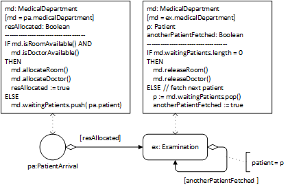
This process model defines the following two event rules.

ON pa: PatientArrival
md : MedicalDepartment resAllocated : Boolean md := pa.medicalDepartment
IF md.isRoomAvailable() AND md.isDoctorAvailable() THEN md.allocateRoom(); md.allocateDoctor(); resAllocated := true ELSE md.waitingPatients.push( pa.patient); resAllocated := false
IF resAllocated SCHEDULE Examination( patient:=pa.patient, medicalDepartment:=md)

ON ex: Examination
md : MedicalDepartment anotherPatientFetched : Boolean p: Patient md := ex.medicalDepartment
IF md.waitingPatients.length = 0 THEN md.releaseRoom(); md.releaseDoctor(); anotherPatientFetched := false ELSE p := md.waitingPatients.pop(); anotherPatientFetched := true
IF anotherPatientFetched SCHEDULE Examination( patient:=p, medicalDepartment:=md)

Notice that the event scheduling arrows of Figure 7-12, and also the SCHEDULE statements of the corresponding event rule tables, do not contain assignments of the duration of activities, since it is assumed that, by default, whenever an activity type has an operation duration(), the duration of activities of this type are assigned by invoking this operation.

A general model with resource objects as members of resource pools

In a more general approach, instead of using resource counter attributes, explicitly modeling resource object classes (like Room and Doctor) allows representing resource roles (stereotyped with «res») and resource pools (stereotyped with «pool») in the form of collections (like md.rooms and md.doctors) and modeling various forms of non-availability of resources (such as machines being defective or humans not being in the shift plan) with the help of corresponding resource status values (such as OUT_OF_ORDER). The result of this elaboration is the information design model shown in Figure 7-13.

For an OE class model, like the one shown in Figure 7-13, the following completeness constraint must hold: when an object type O (like Doctor) participates in a «res» association (a resource role association) with an activity type A (like Examination), the process owner object type of A (MedicalDepartment) must have a «pool» association with O.

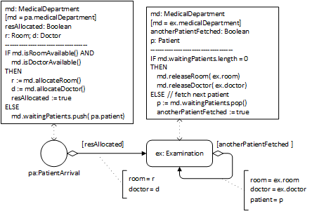
Extending OE Class Diagrams by adding a «resource type» category

The information design model of Figure 7-13 contains two object types, Room and Doctor, which are the range of resource role and resource pool properties (association ends stereotyped «res» and «pool»). Such object types can be categorized as «resource type» with the implied meaning that they inherit a resource status attribute from a pre-defined class Resource, as shown in Figure 7-16.

The introduction of resource types to OEM class models allows simplifying models by dropping the following modeling items from OE class models, making them part of the implicit semantics:

1. the status attributes of object types representing resource types, which are implicitly inherited;
2. the pre-defined enumeration ResourceStatusEL;
3. the resource management operations isAvailable, allocate and release, which are implicitly inherited by any resource type; and
4. the planned activity queues may possibly be implicitly represented for any resource-constrained activity type in the form of ordered multi-valued reference properties of its process owner object type.

This is shown in Figure 7-16.

Revisiting the manufacturing workstation example

A manufacturing workstation, or a "server" in the terminology of Operation Research, represents a resource for the processing activities performed at/by it. This was left implicit in the OE class model shown on the right-hand side of Figure 6-3. Using the new modeling elements (resource types, resource roles and resource pools), the processing activities of a workstation can be explicitly modeled as resource-constrained activities, leading to the OE class model shown in Figure 7-17 and to a more high-level and more readable process model compared to the process model of Figure 6-4.

Decoupling the allocation of multiple resources

In a simplified simulation design for the extended scenario (with patients and nurses first walking to examination rooms before doctors are allocated for starting the examinations) described by the conceptual models of Figure 7-6 and Figure 7-9, we do not consider the walks of doctors, but only the walks of nurses and patients. For simplicity, we drop the superclass people and associate the activity type WalkToRoom with the Patient and Nurse classes. The result of this elaboration is the information design model shown in Figure 7-18.

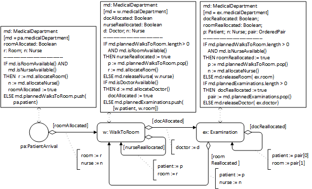
This process design model defines three event rules. Notice that the Examination event rule either re-allocates the doctor to the next planned examination and schedules it, if there is one, or it releases the doctor and re-allocates the room to the next planned walk-to-room and schedules it, if there is one.

Centralizing the re-allocation of resources

As shown before, in the conceptual process models of Figure 7-8 and Figure 7-9, the re-allocation of resources can be centralized with the help of resource release request events and the process owner and the involved performers can be displayed by using a Pool that is partitioned into Lanes for the involved activity performers, resulting in the model shown in Figure 7-20.

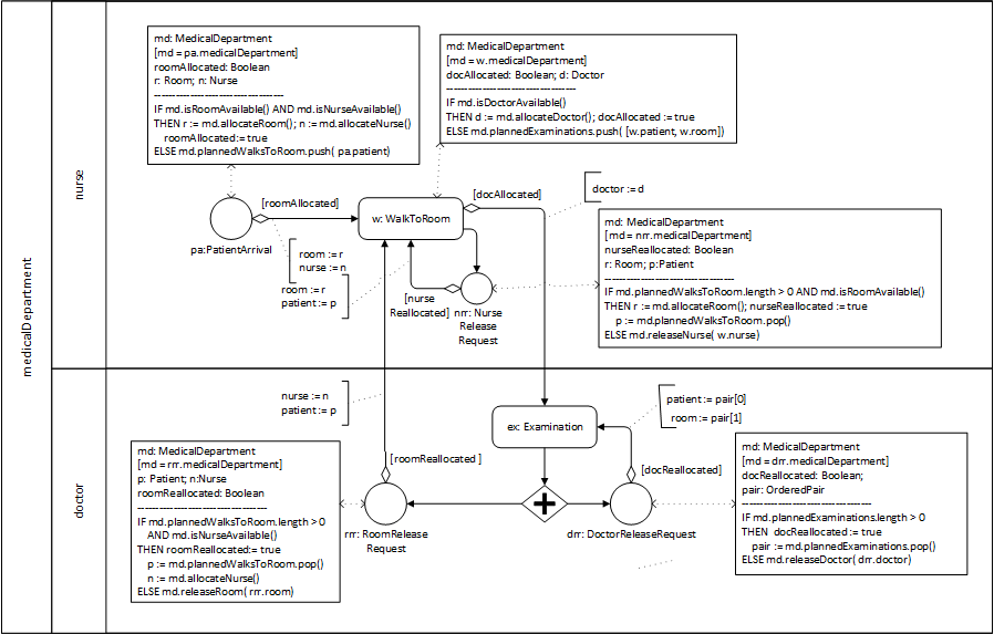
7.3. Introducing Resource-Dependent Activity Scheduling Arrows

The conceptual process model shown in Figure 7-9 and the process design model shown in Figure 7-20 exhibit a general pattern for modeling a sequence of two resource-constrained activities of types A₁ and A₂ shown in Figure 7-21. For describing this Allocate-Release Modeling Pattern, we assume that

1. the process owner maintains queues for planned activities: q₁ for for planned activities of type A₁, and q₂ for planned activities of type A₂, both defined as queue-valued (i.e., ordered multi-valued) reference properties of the process owner in the underlying information model;
2. the underlying information model specifies the sets of resources R₁ and R₂ required by A₁ and A₂;
3. the set of resources required by A₂ but not by A₁ is denoted by R₂−R₁;
4. the set of resources required by A₁ and by A₂ is denoted by R₁∩R₂.

We can describe the execution semantics of the Allocate-Release Modeling Pattern for the case of a succession of an activity of type A₁ by another activity of type A₂ in the following way:

1. ON start event:
   1. If the resources R₁ required by A₁ are available, they are allocated; otherwise, a planned A₁ activity is added to the task queue q₁.
   2. If the resources R₁ have been allocated, a new activity of type A₁ is started.
2. WHEN an activity of type A₁ is completed:
   1. If available, the resources R₂−R₁ are allocated; otherwise, a planned A₂ activity with reserved resources R₁∩R₂ is added to the task queue q₂.
   2. If R₂−R₁ have been allocated, a new activity of type A₂ (with resources R₂−R₁ and R₁∩R₂) is started. In addition, the release of R₁−R₂ is requested.
3. ON release request for R₁−R₂:
   1. If q₁ is not empty and the resources R₁∩R₂ required by both A₁ and A₂ are available, they are allocated and R₁−R₂ are re-allocated to head( q₁); otherwise, R₁−R₂ are released.
   2. If the resources R₁−R₂ have been re-allocated, a new activity of type A₁ is started.
4. WHEN an activity of type A₂ completes:
   1. There is no state change.
   2. An immediate release request for R₂ is caused/scheduled.
5. ON release request for R₂:
   1. If R₁∩R₂ is nonempty: if q₁ is not empty and the resources R₁−R₂ required by A₁, but not yet allocated, are available, they are allocated and R₁∩R₂ are re-allocated to head( q₁); otherwise, R₁∩R₂ are released. If q₂ is not empty, then re-allocate R₂−R₁ to head( q₂); otherwise, R₂−R₁ are released.
   2. If R₁∩R₂ have been re-allocated, a new activity of type A₁ is started. If R₂−R₁ have been re-allocated, a new activity of type A₂ is started.

Since the Allocate-Release Modeling Pattern defines a generic algorithm for scheduling resource-constrained activities as well as allocating and releasing resources, its (pseudo-)code does not have to be included in a DPMN Process Diagram, but can be delegated to an OE simulator supporting the resource-dependent scheduling of resource-constrained activities according to this pattern. This approach allows introducing new DPMN modeling elements for expressing the Allocate-Release Modeling Pattern in a concise way, either leaving allocate-release steps completely implicit, as in the DPMN Process Diagram of Figure 7-22, or explicitly expressing them, as in Figure 7-23.

The most important new DPMN modeling element introduced are Resource-Dependent Activity Scheduling (RDAS) arrows pointing to resource-constrained activities, as in Figure 7-22. These arrows are high-level modeling elements representing the implicit allocate-release logic exhibited in Figure 7-21. Thus, the meaning of the model of Figure 7-22 is provided by the model of Figure 7-21.

It is an option to display the implicit allocate-release steps with Allocate and Release rectangles together with simple control flow arrows, as between the start event circle and the Allocate R1 rectangle in Figure 7-23.

The meaning of the model of Figure 7-23 is the same as that of Figure 7-22, which is provided by the model of Figure 7-21. The fact that, using RDAS arrows, the allocate-release logic of resource-constrained activities does not have to be explicitly modeled and displayed in a process model shows the power of founding a process model on an information model, since the entire resource management logic can be expressed in terms of resource roles, constraints and pools in an information model. This is in contrast to the common approach of industrial simulation tools, such as Simio and AnyLogic, which require defining resource roles, constraints and pools as well as explicit allocate-release steps in the process model, in a similar way as shown in Figure 7-23.

Example 1: Simplifying the workstation process model

We can now simplify the workstation model using the resource type category for WorkStation in the OE class model and a resource-dependent activity scheduling arrow from the arrival event to the processing activity in the DPMN process model. The resulting class model is shown in Figure 7-26.

The simplification of the process model of Figure 6-5 results in the model of Figure 7-25.

Example 2: Simplifying the medical department process model

We can now simplify the medical department model using the resource type category for Doctor, Room and Nurse in the OEM class model and resource-dependent activity scheduling arrows in the DPMN process model. The resulting class model is shown in Figure 7-26.

The simplification of the rather complex process model of Figure 7-20 by using resource-dependent activity scheduling arrows results in the model of Figure 7-27.

7.4. Organization Modeling Concepts

The activities of a business process are typically performed by human resources holding certain organizational positions that authorize them to play certain organizational roles within an organization or organizational unit. It is, therefore, natural that Activity-Based DES modeling includes organization modeling concepts. In particular, the concept of resource roles and the related concepts of organizational roles and organizational positions are paramount to Activity-Based DES modeling.

Many resource modeling concepts, such as resource roles (including performer roles) and resource pools, can be captured in information models in the form of categorized ("stereotyped") UML class modeling elements such as «rr» for resource role association ends, «pr» for performer role association ends, and «rp» for resource pool association ends, leading to an extension of UML Class Diagrams, called OE Class Diagrams, such as the following one:

This conceptual OE class model describes two activity types, "walks to rooms" and "examinations", each one associated with

1. the object type "medical departments", providing the (business) process owner; implying that each specific walk-to-room or examination activity is performed by human resources of, and within a business process owned by, that department;
2. a performer object type ("nurses" or "doctors") via a performer role («pr») association end, providing the activity performer (as a special type of resource);
3. another resource object type via a resource role («rr») association end, providing another resource of each activity (a "room").

In addition, the model describes three types of resource pools by means of «rp» association ends, such that each resource pool is associated with a process owner maintaining the pool and providing the resources corresponding to one of the three resource roles.

Notice that in a conceptual OE class model, each activity type should have a performer role («pr») association, while in an OE class design model (being part of a simulation design model), it is an option to abstract away from the distinction of performers among the resources of an activity and simply consider all its resources (including its performer) as plain resources. This is common in management science and Operations Research, where the main interest is in obtaining general performance statistics for resources, such as their utilization, no matter if they are active resources (performers) or not.

We show how further organization modeling concepts can be introduced to OEM&S.

Refining Object Types to Resource (Role) Types and Performer (Role) Types

While a resource role of an activity type denotes an association end, corresponding to a reference property of the class implementing the activity type, a resource (or performer) role type denotes an object type that is the range of a resource (or performer) role. For simplicity, we say "resource type" (or "performer type") instead of "resource role type" (or "performer role type").

For all «object type» classes of an OE class model that are the range of a performer role or a resource role, it may be an option to replace their «object type» category with a «performer type» or «resource type» category, as shown for the object types "nurses", "doctors" and "rooms" in the following refined model:

Notice that typically each resource type is the range of one resource role and represents a resource pool for it. A resource type may be the target class of more than one resource role association end and its population may be segmented into several resource pools such that at least one pool is assigned to each resource role.

However, the replacement of the «object type» category of a class with a (performer or resource) role type category is only an option, if all instances of the class are playing that role. In the above example, if there are doctors who do not perform examinations (but only surgical operations), then the object type "doctors" cannot be turned into a performer type "doctors" for examinations, but would have to be partitioned into two subtypes, "surgeons" and "examination doctors", such that the latter would be a performer type for examinations.

In OEM&S, a human performer type is implicitly a subtype of the pre-defined object type Person. This makes it possible that a doctor, as a person that performs examinations, may also be a patient in an examination (of course, with the constraint that a person cannot be the same examination's doctor and patient).

Refining Performer Types to Organizational Positions

An organizational position is defined by a name and a set of human performer types representing the roles of the position holders. For instance, in a medical department, the organizational position Nurse may be defined by the set of performer types Guide and ExaminationAssistant, where a Guide is required for guiding a patient to an examination room and an ExaminationAssistant is required for assisting a doctor in a medical examination.

Computationally, an organizational position is an object type that is co-extensional with all of its performer types, implying that its instances (position holders) are human resources that can be allocated for performing any activity associated with any of these performer types. This implies that any instance (or "holder") of an organizational position is a person and that any organizational position is a subtype of the kind Person.

For instance, the organizational position Nurse is co-extensional with the performer types Guide and ExaminationAssistant, with the meaning that nurses may play the role of guides or the role of examination assistants, and any guide, as well as any examination assistant, is a nurse.

In simple cases, an organizational position is defined by just one performer type for one particular performer role.

In OEM&S, for each organizational position (like Clerk) consisting of the performer roles p₁,...,p_n, there is a default resource pool, or better: performer pool, (like clerks) that includes all employees holding that position. This pool will be used for allocating the performers of activities with a performer role p_i.

These considerations lead to the following refined version of the medical department model shown in the diagram above:

Notice that in this refined model, we have also categorized the object type "patients" as «person role type» and the object type "medical departments" as «organizational unit type». In OEM&S, a person role type, like Patient, is implicitly a subtype of the pre-defined object type Person, allowing a doctor to be a patient. An organizational unit, as an instance of an organizational unit type, may own one or more business processes.

Assigning business process types and business goals to organizational agents

An organizational agent, which is either an organization, an organizational unit or an organizational role player, can own business process types and can have business goals, which allow improving business processes by refactoring business process models, including resource allocation policies, and by changing the populations of resource pools, in such a way that the goals of the process owner (and those of its super-agents) are satisfied.

Consider the following example:

There are different ways of expressing business goals. In simulation modeling, we need operational forms of business goals, that is, expressions in a formal language. We consider three forms of business goals:

1. Definite goals (like "raise the overall revenue by at least 25%") are defined by a logical condition (like relativeRevenueRise >= 0.25) that can be checked by a simulator.
2. Variable change goals are defined by a combination of one of the verbs "increase" or "decrease" with the name of a variable (like "profit", "customer satisfaction" or "costs").
3. Optimization goals are (more ambitious) special variable change goals defined by a combination of one of the verbs "maximize" or "minimize" with the name of a variable (like "profit", "customer satisfaction" or "costs").

7.5. Resource Modeling

Whenever an activity of a certain type is to be performed, various resources may be required for performing it and have to be allocated first. We can distinguish between ‘active’ (or performer) resources, such as human resources, robots or IT systems, which execute activities, and ‘passive’ resources, such as rooms or devices, which are used by performers for executing activities.

Business process models focus on describing the possible sequences of events and activities, based on conditional and parallel branching. But they may also describe resource roles, which associate resources of a certain type with activities of a certain type.

In the field of Business Process Management (BPM), there is a tendency to consider workflow processes as paradigmatic for business processes. However, workflow processes typically only have (human) performer resources, while business processes in general often have one or more passive resources in addition to a performer. Due to this tendency, BPM research often adopts a simplistic view of business processes.

E.g., in (Pufahl et al. 2021), resource allocation is defined as the “assignment of a process task to the most appropriate resource”, while in general, it’s the other way around: resources are assigned to a task. The authors also point out that the vast majority of BPM research studies on resource allocation make the assumption that a task requires just one resource and a resource cannot be used in more than one task at the same time. As opposed to this simplistic view of business processes in BPM, in DES, tasks can have more than one required resource, and resources may be used in more than one task at the same time.

It is important to distinguish between the passive resources required for performing an activity and the inputs required for performing a processing (or transformation) activity. While the passive resources used in an activity survive the activity, and can be reused in the next one, inputs are either processed, or transformed, into outputs of the activity, and cannot be reused for the next activity. In the literature, this conceptual distinction is often not made. Instead, e.g., in (Russell et al. 2004; Goel and Lin 2021), processing activity inputs are called ‘consumable resources’. However, resources cannot be ‘consumed’, but they can be worn out by activities, such that if their degree of wear falls below a certain threshold, they can no longer be used and are depleted.

For various reasons, resources can go out of order: machines may fail or may have to get scheduled maintenance, nurses or doctors may get sick or may be out-of-duty or off-shift. Consequently, both planned and unexpected resource outages may have to be modeled.

7.5.1. Resource Cardinality Constraints and Multitasking Constraints

Since activities require resources, and resources are allocated to planned activities, it is crucial to understand the relationship between activities and resources. An important part of its meaning are resource cardinality constraints and multitasking constraints.

Business process models do not only describe the possible sequences of events and activities, but they also describe the dependency of activities on resources. For instance, in a BPMN process diagram, a Lane L (such as the doctors lane in the BPMN process diagram below) may represent a resource type such that the diagram specifies for any Activity rectangle A in L (such as examinations) that an activity of type A is performed by a resource of type L.

While using a container shape, such as a BPMN Lane, for assigning elements, such as activities, to the element represented by the container shape (viz, a resource role) is a good way of visually expressing a many-to-one relationship between activity types and resource roles (all activity types within a Lane do have exactly one resource role), it does not allow expressing one-to-many or many-to-many relationships between activity types and resource roles.

Therefore, the BPMN Lane notation can only be used for specifying a performer resource role for activities that do not require resources of other types, and where we have a one-to-one association: (1) a resource can be allocated to at most one activity, and (2) an activity is performed by exactly one resource.

In general, though, the relationships between activities (of some type) and resources (of some type) can be best described by binary relationship types in an information model, such as by binary associations in a UML class diagram with multiplicity expressions at both ends. Figure 7-29 shows two one-to-one associations between the activity type examinations and the object types rooms and doctors associating a room as a (passive) resource and a doctor as a performer resource to an examination activity.

The association end at the side of the object type doctors is categorized as a resource role with the help of UML’s stereotype notation. The multiplicity expression at the resource role end is called resource multiplicity. In our example, the resource multiplicity at the doctors end is ”1” (an abbreviation of "1..1"), which means that exactly one doctor is required for performing an examination, defining a resource cardinality constraint that is a conjunction of a minimum resource cardinality constraint ("at least one") and a maximum resource cardinality constraint ("at most one").

In general, a multiplicity expression defines both a lower bound and an upper bound. When the lower bound of a resource multiplicity is greater than 0, it defines a minimum resource cardinality constraint. When the upper bound of a resource multiplicity is a natural number greater than 0, it defines a maximum resource cardinality constraint. The resource multiplicity 0..* (where * stands for unbounded), which does not define any resource cardinality constraint, is rather unusual since normally all activities require at least one resource (their performer).

The multiplicity of the association end at the other side (of the activity type) represents a multitasking constraint, which defines if a resource is exclusively allocated to an activity, or to how many activities a resource can be allocated at the same time. In our example, the multiplicity 0..1 represents a multitasking constraint stating that, at any point in time, a doctor can be associated with, or perform, either no examination or at most one examination.

In an Object-Oriented (OO) programming approach, the computational meaning of a resource role is provided by a corresponding property in the class implementing the activity type. In the above example, the resource role association of "examinations" with "doctors" leads to a property doctor in the class Examination, as shown in Figure 7-30.

When activities admit using more resources than required, this means they can be started as soon as the required number of resources are available, but they can also be started with a greater number of resources, typically implying a faster performance.

While the model shown in Figure 7-29 is an example of a one-to-one association between an activity type and a resource object type, which is the only option in BPMN process models, we consider the cases of one-to-many, many-to-one and many-to-many associations in the following subsections.

One-to-Many Relationships

An example of a one-to-many relationship between activity types and resource object types is the association between ”load truck” activities and ”wheel loader” resources shown in Figure 7-31.

Notice that in this diagram, the «resource role» designation of the association end at the side of “wheel loaders” has been abbreviated by the keyword «rr». Its resource multiplicity of 1..2 specifies a minimum resource cardinality constraint of “at least one” and a maximum resource cardinality constraint of “at most two”, meaning that one wheel loader is required and a second one is admissible. When an activity does not require, but admits of, using more than one resource (of the same type), this typically means that the duration of the activity is the more decreasing the more resources are being used.

The one-to-many resource role association of ”load truck” with ”wheel loaders” leads to a property wheelLoaders in the activity class LoadTruck, as shown in Figure 7-32. Notice that this property has the multiplicity 1..2, which means that it is collection-valued and has either a singleton or a two-element collection value.

When activities admit using more resources than required, this means they can be started as soon as the required number of resources are available, but they can also be started with a greater number of resources, typically implying a shorter duration.

Many-to-One Relationships

An example of a many-to-one relationship between activity types and resource object types is the association between ”examination” activities and ”examination room” resources shown in Figure 7-33.

In this example, examination rooms (as resources) admit of up to three examinations being performed at the same time. Such a multitasking constraint can be implemented with the help of a (multitasking) capacity attribute of the class implementing the resource object type. If such a constraint applies to all instances of a resource object type, capacity would be a class-level (”static”) attribute, which is rendered underlined in a UML class diagram, as shown in the following model:

Alternatively, if different examination rooms have different capacities, then capacity would be an ordinary (instance-level) attribute of the class ExaminationRoom.

Many-to-Many Relationships

Examples of many-to-many relationships between activity types and resource object types are rare and typically involve activities going on with interruptions. An example is the association between ”teaching a course” activities and ”teacher” resources shown in Figure 7-34. In this example, the teaching of a course admits at most two teachers who may be involved in at most 7 course teaching activities at the same time.

7.5.2. Organizational Positions and Resource Pools

Since a business process happens in the context of an organization, it is natural to consider the concept of organizational positions, which has been introduced in Section 7.4.

Resource roles (including performer roles), resource types (including performer types), organizational positions and resource pools are defined in an OE class model. A resource role of an activity type is a special type of property having a resource type as its range.

A performer role of an activity type has a performer type as its range. For instance, in the following OE class model, the (implicitly named) performer role orderTaker of the activity type TakeOrder has the performer type OrderTaker as its range. Likewise the object type PizzaMaker is a performer type. A performer type may be an organizational position. For instance, in the following OE class model, both OrderTaker and PizzaMaker are organizational positions, for which an organization hires a number of human resources, forming corresponding resource pools (called orderTakers and pizzaMakers). These resource pools correspond to the direct populations of the two organizational positions.

An organizational position may subsume more than one performer role. In the model above, the organizational position PizzaMaker is an alternative resource subtype of the organizational position OrderTaker, as indicated by the generalization arrow with the category keyword «ar» (a UML "stereotype").

When a resource pool represents an organizational position charged with playing n performer roles, it is used by all n corresponding activity types.

It is an option that the resources of an alternate resource pool, corresponding to an alternative resource subtype, are associated with a lower proficiency level increasing both the duration of activities and their rework probabilities.

7.5.3. Alternate Resource Pools

Certain activities allow alternative resources, when no standard resources are available. For instance, in a pizza service company, when no order taker is available, and a new order call comes in, an available pizza baker can take the order. Or in a hospital, where nurses guide patients to an examination room, when no nurse is available, a receptionist can guide a patient to an examination room.

The general conceptual pattern is that for certain types of activities A (like GuideToRoom), a resource role r (like guide) may be played not only by instances of its direct resource type R (like Guide), but also by instances of an alternative resource type R' (like ExaminationAssistant) or an organizational position P (like Nurse), if they are a subtypes of R (Guide).

When the resource type R is not abstract, then its instances are the preferred resources of activities of type A, and its (possibly preference-rank-annotated) alternate resource subtypes specify types of alternative resources.

By default, for any non-abstract resource type R and for any organizational position P assigned as the range of a resource role r, an OE simulator can create a resource pool with the same (yet pluralized) name, pooling objects instantiating R or P, and assign it to r as the preferred resource pool.

An alternate resource pool can be defined in an OE class model by means of an alternate resource subtyping arrow (a UML generalization arrow designated with «ar») between the alternative resource type and the resource type concerned as shown in the following diagram, where PizzaMaker is modeled as an alternative resource subtype of OrderTaker:

7.5.6. Resource Outages

For various reasons, resources can go out of order: machines may fail or may have to get scheduled maintenance, nurses or doctors may get sick or may be out-of-duty or off-shift. Consequently, both planned and unexpected resource outages may have to be modeled.

While human resources being out-of-duty or off-shift can be modeled with the help of service time calendars, scheduled maintenance may be modeled in the form of maintenance activities recurring with a fixed interval. Unexpected resource outages are resource failures.

Modeling Resource Failures

Resource failures can be modeled with the help of two types of events: failure and recovery, and two related random variables: time-to-next-failure and failure time. In this approach, the next resource failure event occurs x time units after a recovery event, where x is obtained by invoking the random variable sampling function timeToNextFailure(). Each failure event triggers a recovery event, which is scheduled with a delay of y time units where y is obtained by invoking the random variable sampling function failureTime().

This simple approach applies both to non-human and human resources.

Further modeling options:

• Allow specifying a time-to-first-failure, in addition to the time-to-next-failure.
• Allow counting only the busy time of a resource, instead of the total time, for determining its next failure time.

Modeling the Repair of Failed Resources

In activity-based simulation, the basic failure modeling approach can be refined by modeling the repair of a failed non-human resource as an activity whose duration is provided by the random variable repair time and which requires a repair person as a resource, such that the total failure time is the sum of the two random variables repair lead time (the time needed for getting a repair person to start the repair) and repair time.

Then, when a failure event occurs, it triggers a repair activity to start with a delay of x time units and a duration of y time units, where x = repairLeadtime() and y = repairTime(). The next failure event is scheduled to occur z time units after a repair end event, where z is obtained by invoking the random variable sampling function timeToNextFailure().

Modeling the Scheduled Maintenance of Resources

Non-human resources, such as machines, may undergo periodic maintenance for preventing them to fail in the near future. This can be modeled by scheduling periodic maintenance activities every x time units where x = maintenanceIntervall(), along with periodic failure events.

When a maintenance activity starts before the next scheduled failure event has occurred, the simulator has to retract this event from the Future Event List for implementing its prevention by the maintenance activity. The next failure event is scheduled to occur x time units after the maintenance end event, where x is obtained by invoking the random variable sampling function timeToNextFailure().

When a resource fails before its next scheduled maintenance has started, the scheduled maintenance is cancelled (the simulator has to retract the scheduled maintenance start event) and, instead, the failure event triggers a repair activity. Only when the repair activity ends, the next maintenance activity is scheduled with a delay of y time units where y is obtained by invoking the random variable sampling function maintenanceTime().

Further modeling options:

• Allow specifying a time-to-first-maintenance, in addition to the maintenance interval time-to-next-maintenance.
• Allow specifying the recurrence of maintenance activities with a schedule instead of a (typically fixed) maintenance interval.

Defining General Elements for Modeling Resource Outages

A simulation framework/language should support resource outage modeling by allowing to define for each (non-human) resource object type the three pairs of (typically random variable) time functions introduced above and summarized in the following class diagram.

These pairs of time functions have to be used incrementally: specifying maintenance time functions requires specifying repair time functions, which, in turn, requires specifying failure time functions.

Resource Outage Modeling in AnyLogic

AnyLogic is a state-of-the-art DES modeling tool/framework. It allows defining recurrent failures (not with follow-up recovery events, but only with follow-up repair activities) and maintenance for each Resource Pool. There is the option to use only the busy time of a resource for computing its next failure time. For repair activities, there is no possibility to distinguish between repair lead time and repair time. For maintenance activities, it can be defined which task priority they have and if they are preemptive or not. Neither for repair nor for maintenance activities, performer resources can be assigned.

10.1. Perception and Action

Agents may perceive objects and events in their environment and, in response, take certain actions, possibly causing changes in their environment.

One can distinguish between a passive and an active form of perception. Passive perception takes place asynchronously, while an agent is busy or idle, in the form of (instantaneous) perception events, while active perception requires the agent to perform a perceptive action or activity (like scanning the neighborhood). In general, agents are exposed to perception events and may react in response to them.

In the case of physical agents, like robots, passive perception events are created by a sensor containing an event detector, such as a Proximity Infra-Red (PIR) sensor, which has its output pin going high whenever it detects an infra-red emitting object (e.g., a human or a medium to large sized animal) in its reach. Active perceptions are created by querying the measurement value of a sensor containing a quality detector, such as a DHT22 temperature and humidity sensor. The distinction between event detectors and quality detectors has been proposed in (Diaconescu and Wagner 2015).

Perception events typically lead to an update of existing beliefs or to the creation of new beliefs.

10.2. Communication

There are various forms of communication between agents. In particular, we can distinguish between verbal and non-verbal communication. We are only concerned with verbal communication, which is based on messages.

Ontological Considerations

Conceptually, a communication event is composed of two successive atomic events: an out-message event (corresponding to a send message action of the sender) and a correlated in-message event (or message reception by the receiver). This is illustrated by the following diagram:

This concept diagram expresses the following ontological stipulations:

• A message is sent from a sender agent to one or more receiver agents via an out-message event.

• A message from a sender agent is received by a receiver agent via an in-message event.

• A communication event consists of a pair of correlated out/in message events out and in, such that the following conditions hold:

  • in.message = out.message
  • in.receiver is included in out.receivers
  • in.sender = out.sender
  • in.occurrenceTime > out.occurrenceTime

Communication events may lead to updates (and deletions) of existing beliefs or to the creation of new beliefs, especially in information exchange processes based on Tell-Ask-Reply messages.

Message Types

Each message is of a certain type defining its properties and implicit semantics. There are two kinds of message types:

1. User-defined problem/domain-specific message types: the structure of such a message type is defined within a simulation model in the form of a class defining its properties; their semantics is defined in the receive methods of receiver agents in terms of how messages of such a type are processed.
2. Pre-defined problem/domain-independent message types: Tell and Ask/Reply are examples of problem/domain-independent message types that may be supported by a simulator. As they refer to general speech acts, the semantics of these message types should be based on the philosophical speech act theory of Austin and Searle.

There are two prominent agent communication language standards: FIPA and KQML (Finin et al 1997), both defining domain-independent standard message types with a semantics based on speech act theory. We briefly describe the rules for processing Tell, Ask, Reply and Request messages:

Tell

Using this message type, agents may communicate some of their beliefs to other agents, without being asked. In general, a teller may tell the truth or may lie; and in both cases the provided information may or may not be correct.

A Tell message is similar to what is called a Signal in the Unified Modeling Language (UML) where a Signal is sent asynchronously from an object to another object. The event rule for processing a Signal reception event is defined by specifying a Reception operation in the classifier of the receiver object, such that this operation has the same name as the type of the Signal (and a corresponding signature). We do not use these UML concepts (and the UML terminology) since they are too limited.

Ask

Using this message type, an agent may query another agent about some of its beliefs. Queries are expressed in a suitable query language, such as the RDF-based query language SPARQL. An asker expects to receive an answer via a Reply message some time later.

Reply

This message type is used for replying to a previously received Ask message. In general, the answers provided may or may not be correct. Therefore, askers should only update their beliefs according to the received answers when they trust the replier.

Request

This message type is used by an agent for requesting another agent to perform a certain action. Such a request can be either accepted or rejected.

Since a perfect information agent already has complete information about the objects it knows,

• sending a query via an Ask message only makes sense if the query may retrieve objects the sender does not yet know;
• sending an answer via a Reply message only makes sense if the answer provides information about objects the receiver does not yet know;
• receiving a statement via a Tell message only makes sense if the statement provides information about an object the receiver does not yet know.

10.3. Interleaved Agent Simulation

In interleaved agent simulation, the simulator processes a PerceptionEvent by invoking the method onPerceive of the perceiver agent. An agent performs an action, e.g., in response to a perception, with the help of its perform method, which schedules a corresponding ActionEvent that is then processed by the simulator.

Likewise, message-based communication is implemented by having the sender agent invoking its send method, which schedules a MessageEvent that is then processed by the simulator by invoking the onReceive method of the receiver agent. In this way, a MessageEvent is inserted into the simulation log and it is guaranteed that, as required above, the time when a message is received is later than the time it has been sent (in.occurrenceTime > out.occurrenceTime).

Perception and Action

For supporting perception events and actions, the OEM&S concept Event is extended in the following way:

This means that

1. The pre-defined (abstract) object type Agent has two abstract methods for perception and action:
   1. onPerceive to be invoked with a perception argument, which is a PerceptionEvent,
   2. perform to be invoked with an action argument, which is an Action.
2. There are two pre-defined (abstract) event types: PerceptionEvent and Action.
3. A PerceptionEvent has a perceiver reference and may have additional attribute values.
4. When a PerceptionEvent is processed by the simulator, it invokes the onPerceive method of the perceiver agent and passes the perception (event). This implies that the code for realizing the effects of a perception event is included in the agent class (in its definition of the onPerceive method).
5. An Action event has a performer reference and may have additional attribute values.
6. When an agent performs an action by invoking the perform method, an Action event is scheduled, which is then processed by the simulator by invoking the onEvent method defined in the action event class. This implies that the code for realizing the effects of an action is included in the action event class (in its definition of the action event handler onEvent).

Message-Based Communication

The following diagram shows the new A/OEM&S elements added to the OEM&S meta-model:

This means that

1. The pre-defined (abstract) class Agent has the abstract method onReceive to be invoked with a message and a sender reference.
2. There is a pre-defined event type MessageEvent.
3. A MessageEvent has a message attribute value, which is a string or a composite value.
4. When a MessageEvent occurs, the simulator invokes the onReceive method of the receiver agent and passes the message attribute value. This implies that the code for realizing the effects of an in-message event is included in the agent class (in its definition of the onReceive method).

In a distributed simulator for A/OEM&S, where all agents of a simulation scenario run as different processes (on different computers) without a shared simulator state, and, consequently, message passing would be asynchronous, it would be natural to implement both out-message events and in-message events, as described above.

Agent-Based Simulation with OESjs

Typically, a sender agent sends a message (or schedules a MessageEvent) within its onPerceive or onReceive methods, that is, in response to a perception or to a message reception. In OESjs-Core4, this could be programmed in the following way:

1
2
3
4
5
6
7
8
9
10
11
12
13
14
15
16
17
18

class Doctor extends aGENT {
  constructor({ id, name, status}) {
    super( id, name);
    this.status = status;
  }
  onReceive( msg, sender) {
    switch (msg.type) {
    case "ASK": 
      const answer = this.processQuery( msg.query),
            reply = new rEPLY( answer),
            receiver = sender;
      this.send( reply, receiver));
      break;
    case "REPLY":
      ... 
    }
  }
}

Often, a PerceptionEvent is scheduled as a consequence of an action event with the meaning that the action is perceived by another agent. A PerceptionEvent is processed by the simulator by invoking the onPerceive method of the perceiver agent while passing the perception attribute value.

An Action is typically performed by an agent within its onPerceive or onReceive methods in response to a perception or to a message reception. In OESjs, this could be programmed in the following way:

1
2
3
4
5
6
7
8
9
10
11
12
13

class Doctor extends aGENT {
  constructor({ id, name, status}) {
    super( id, name);
    this.status = status;
  }
  onPerceive( perceptionEvt) {
    switch (perceptionEvt.constructor.name) {
    case "CovidSymptom":
      this.perform( new aCTION("performPCR"));
      break;
    }
  }
}

Bibliography

- Aalst, Wil M. P. van der. 2021. "Concurrency and Objects Matter! Disentangling the Fabric of Real Operational Processes to Create Digital Twins". In A. Cerone and P. C. ̈Olveczky (Eds.): Proceedings of International Colloquium on Theoretical Aspects of Computing (ICTAC 2021), LNCS 12819, pp. 3–17.
- Allen, G.N., and S.T. March. 2003. Modeling temporal dynamics for business systems. Journal of Database Management, 14, 21–36.
- Almeida, J.P.A., R. Falbo and G. Guizzardi. 2019. Events as Entities in Ontology-Driven Conceptual Modeling, in Proceedings of 38th International Conference on Conceptual Modeling, ER 2019, Salvador, Brazil, November 4–7, 2019.
- Diaconescu, M. and G. Wagner. 2015. Modeling and Simulation of Web-of-Things Systems Part 1: Sensor Nodes. In L. Yilmaz, W. K. V. Chan, I. Moon, T. M. K. Roeder, C. Macal and M. D. Rossetti (Eds.), Proceedings of the 2015 Winter Simulation Conference. pp. 3061–3072. Piscataway, New Jersey: Institute of Electrical and Electronics Engineers. http://www.informs-sim.org/wsc15papers/300.pdf
- Casati, R., and A. Varzi, Events, in: E.N. Zalta (Ed.), The Stanford Encyclopedia of Philosophy, 2015.
- Chen, P. 1976. The entity-relationship model – toward a unified view of data. ACM Transactions on Database Systems, 1(1):9–36.
- Fine, K. 2022. Acts and embodiment, Metaphysics, 5:1, 14–28.
- Finin T., Y. Labrou and J. Mayfield. 1997. KQML as an agent communication language. In J. Bradshaw (Ed.), Software Agents, MIT Press, Cambridge.
- Gordon, G. 1961. A general purpose systems simulation program. In AFIPS '61: Proceedings of the Eastern Joint Computer Conference, 87–104, New York: Association for Computing Machinery.
- Griffo, C., J.P.A. Almeida, G. Guizzardi, and J.C. Nardi. 2021. Service contract modeling in Enterprise Architecture: An ontology-based approach, Information Systems 101.
- Guarino, N., and G. Guizzardi. 2024. Processes as variable embodiments. Synthese vol. 203, article no. 104. https://doi.org/10.1007/s11229-024-04505-2
- Guarino, N., and C. Welty. 2009. An Overview of OntoClean. In Handbook on Ontologies. https://doi.org/10.1007/978-3-540-92673-3_9.
- Guizzardi, G. 2005. Ontological Foundations for Structural Conceptual Models. PhD thesis, CTIT PhD Thesis Series, No. 05-74 Telematica Instituut Fundamental Research Series, No. 015 (TI/FRS/015).
- Guizzardi, G., A. Botti Benevides, C. M. Fonseca, D. Porello, J. P. A. Almeida, and T. P. Sales. 2022. UFO: Unified Foundational Ontology, Applied Ontology 17, 1–44.
- Loch C.H. 1998. Operations Management and Reengineering, European Management Journal 16, pp. 306–317.
- March, S., and G. Allen. 2009. Conceptual Modeling of Events for Active Information Systems. In Sugumaran, V. (Ed.). Distributed Artificial Intelligence, Agent Technology, and Collaborative Applications. IGI Global. https://doi.org/10.4018/978-1-60566-144-5
- Markowitz, H., B. Hausner, and H. Karr. 1962. SIMSCRIPT: A Simulation Programming Language. Englewood Cliffs, N. J.: Prentice Hall. Available from https://www.rand.org/content/dam/rand/pubs/research_memoranda/2009/RM3310.pdf
- McCarthy, W.E. 1979. An Entity-Relationship View of Accounting Models. The Accounting Review, Vol. LIV, No. 4.
Pegden, C.D. and D.A. Davis. 1992. “Arena: a SIMAN/Cinema-Based Hierarchical Modeling System”. In Proceedings of the 1992 Winter Simulation Conference, edited by J.J. Swain, D. Goldsman, R.C. Crain, and J.R. Wilson, 390–399. Piscataway, New Jersey: Institute of Electrical and Electronics Engineers, Inc.
- Pegden, C.D. 2010. “Advanced Tutorial: Overview of Simulation World Views”. In Proceedings of the 2010 Winter Simulation Conference, edited by B. Johansson, S. Jain, J. Montoya-Torres, J. Hugan, and E. Yücesan, 643−651. Piscataway, New Jersey: Institute of Electrical and Electronics Engineers, Inc. Available from http://www.informs-sim.org/wsc10papers/019.pdf
- Petri, C. A. 1962. Kommunikation mit Automaten. Ph. D. thesis, Institut für Instrumentelle Mathematik, Bonn. English Translation, 1966: Communication with Automata, Technical Report RADC-TR-65-377, Rome Air Development Center, Air Force Systems Command, Griffiss Air Force Base, New York.
- Ross, R.G. 2023. Rules: Shaping Behavior and Knowledge. Business Rule Solutions, LLC.
- Russell, N., A. H. ter Hofstede, D. Edmond, and W. M. van der Aalst. 2004. Workflow Resource Patterns. http://www. workflowpatterns.com/patterns/resource/, accessed 2022-04-15.
- Schruben, L.W. 1983. Simulation Modeling with Event Graphs. Communications of the ACM 26, pp. 957–963. https://dl.acm.org/citation.cfm?id=358460
- Tauzovich, B. 1991. Toward Temporal extensions of the Entity-Relationship Model. Proceedings of the 10th International Conference on Entity Relationship Approach, San Mateo, California: E-R Institute, pp. 136-179.
- Standridge, C.R. 2013. Beyond Lean: Simulation in Practice, Second Edition, Open Access book, available from https://scholarworks.gvsu.edu/cgi/viewcontent.cgi?article=1006&context=books.
- Vincent, P., K. Iijima, A. Leow, M. West, and O. Matvitskyy. 2022. Magic Quadrant for Enterprise Low-Code Application Platforms. Gartner Report G00759450.
- Wagner, G. 2017. An Abstract State Machine Semantics for Discrete Event Simulation. In Proceedings of the 2017 Winter Simulation Conference. Piscataway, NJ: Institute of Electrical and Electronics Engineers. Available from https://www.informs-sim.org/wsc17papers/includes/files/056.pdf.
- Wagner, G. 2018. Information and Process Modeling for Simulation – Part I: Objects and Events. Journal of Simulation Engineering, vol. 1, 2018. https://articles.jsime.org/1/1.
- Wagner, G. 2022. Object Event Modeling for DES and IS Engineering. Proceedings of the ER Forum 2022. In: Link, S., I. Reinhartz-Berger, J. Zdravkovic, D. Bork and S. Srinivasa (Eds.). volume 3211. CEUR Workshop Proceedings.
- Zeigler, B.P. 1976. Theory of Modeling and Simulation. Wiley, New York.